Article

Rapid Warming in the Australian Alps from Observation and NARCliM Simulations

1
Science, Economics and Insights Division, NSW Department of Planning and Environment, Lidcombe, NSW 2141, Australia
2
Australian Research Council Centre of Excellence for Climate Extremes, University of New South Wales, Sydney, NSW 2052, Australia
3
Climate Change Research Centre, University of New South Wales, Sydney, NSW 2052, Australia
4
Département des Sciences de la Terre et de l’Atmosphère, Université du Québec à Montréal, Montreal, QC H3C 3P8, Canada
5
E3-Complexity Consulting, Sydney, NSW 2122, Australia
6
School of Geography, Planning and Spatial Sciences, University of Tasmania, Hobart, TAS 7001, Australia
*
Author to whom correspondence should be addressed.
Atmosphere 2022, 13(10), 1686; https://doi.org/10.3390/atmos13101686
Submission received: 14 September 2022 / Revised: 7 October 2022 / Accepted: 12 October 2022 / Published: 14 October 2022
(This article belongs to the Special Issue Climate Extremes and Their Impacts)

Abstract

:
The Australian Alps are the highest mountain range in Australia, which are important for biodiversity, energy generation and winter tourism. Significant increases in temperature in the past decades has had a huge impact on biodiversity and ecosystem in this region. In this study, observed temperature is used to assess how temperature changed over the Australian Alps and surrounding areas. We also use outputs from two generations of NARCliM (NSW and Australian Regional Climate Modelling) to investigate spatial and temporal variation of future changes in temperature and its extremes. The results show temperature increases faster for the Australian Alps than the surrounding areas, with clear spatial and temporal variation. The changes in temperature and its extremes are found to be strongly correlated with changes in albedo, which suggests faster warming in cool season might be dominated by decrease in albedo resulting from future changes in natural snowfall and snowpack. The warming induced reduction in future snow cover in the Australian Alps will have a significant impact on this region.

1. Introduction

The Australian Alps are the highest mountain range in Australia. The range straddles the borders of eastern Victoria, south-eastern New South Wales, and the Australian Capital Territory (Figure 1). The Alpine region contains Australia’s only peaks exceeding 2000 m in elevation and is the only region in Australian mainland to have annual deep snow, which is important for ecosystem, biodiversity, energy generation and winter tourism.
The Australian Alpine region contains unique Australian ecosystems and iconic species. Australia’s alpine fauna is highly vulnerable to climate change [1]. The mountain pygmy-possum, which is an iconic species, may completely lost their bioclimatic range with a temperature rise of only 1 °C accompanied by a 5% reduction in winter precipitation [2]. Some unique alpine vegetation communities such as short alpine herbfield and snowbank feldmark are also likely to experience distribution changes in the warming climate [3]. The Australian Alps are also important as a winter drainage basin for the Murray, Murrumbidgee, and Snowy River systems. The Snowy Mountains Hydroelectric Scheme, which is a major hydro-energy producer in Australia, artificially collects and diverts runoff from rainfall and snowmelt into the Murray and Murrumbidgee Rivers to generate electricity and provide water resource for the Murray-Darling Basin, which is Australia’s main region for irrigated agriculture. Australia’s major downhill ski resorts are all located in this region. The snow industry is one of the biggest employers in regional Australia, which is important in improving employment outcomes for residents of these regions [4].
Due to relatively low elevations and their latitudinal location, the Australian Alps snow fields are particularly vulnerable to climate change. Brown and Mote [5] identified that mean air temperature over Australian Alps fall within the range of −5 to 5 °C in winter, which has high sensitivity to global warming. Thompson [6] stated, “the Australian Alps are likely to be amongst the first alpine areas in the Southern Hemisphere where the effects of climatic change will be observed”. Data collected from in situ monitoring sites [7,8,9,10] and satellite remote sensing [11,12] have shown the impact of warming in these regions. Several recent studies have investigated the impact of future global warming on snow in the Australia Alps [8,12]. All these studies use Global Climate Model (GCM) simulations to assess climate change in Australian Alps despite the coarse resolution of GCMs cannot capture main characteristics of the alpine region. While GCMs are widely used in large scale climate projections, assessing regional and local changes in temperature and its extremes require finer spatial resolutions and sometimes more processes (e.g., convective storms). Dynamical and statistical downscaling are typically used to bridge the resolution gap and produce high resolution regional climate simulations.
The NSW and Australian Regional Climate Modelling (NARCliM) project is designed to provide plausible future climate conditions for southeast Australia [13]. The first generation of NARCliM (N1.0) was delivered in 2014. A number of studies have evaluated the N1.0 historical simulations [14,15] and shown that N1.0 can simulate observed climate well, even if most of simulations have wet and cold biases. Other studies have also confirmed that N1.0 simulations are better than their driving GCMs in simulating precipitation and temperatures [16]. Since, N1.0 was made available, it has been widely used as a critical data input for climate impact studies, such as assessing changes in rainfall extremes [17,18], extra-tropical low pressure systems [19,20,21], fire-weather and fuel load projections [22,23,24], near surface winds [25], vertical temperature profiles and temperature inversion [26,27], quantifying the impact of urban expansion on local temperature extreme [28,29], assessing future changes in cropping [30,31,32], hydrological impact and wet/dry spells [33] and natural hazards [34].
Whilst the N1.0 simulations are successfully used in many applications, some limitations in the N1.0 experimental design are identified such as older phases of CMIP (Coupled Model Intercomparison Project) GCMs (i.e., CMIP3), non-continuous simulations for three 20-years epochs, and single emission scenario. To address those limitations in N1.0, a second generation of enhanced and updated NARCliM simulations (N1.5 thereafter) were performed.
Designed to complement N1.0, N1.5 provided continuous long-term simulations instead of 20-year periodic simulations provided by N1.0. In the meantime, N1.5 used two out of three RCMs from N1.0 and the same model domains to enable users to choose either or both datasets without consideration of the impacts from change in the boundary and/or regional model physics. In N1.5, 12 sets of regional climate projections were generated by downscaling from three selected CMIP5 GCMs for two Representative Concentration Pathway (RCP8.5 and RCP4.5) [35].
Nishant et al. (2021) [35] and Ji et al. (2022) [36] have evaluated and compared N1.0 and N1.5 in simulating historical mean temperature and precipitation, and climate extremes over southeast Australia. The results indicated that N1.5 performed substantially better than N1.0 in capturing seasonal pattens and magnitudes of precipitation, while its skills for simulating maximum and minimum temperatures were similar to those of N1.0. N1.5 simulations project a hotter and drier future relative to N1.0. N1.0 and N1.5 ensembles provide an improved, more comprehensive data set for studying climate change.
Di Luca et al. (2018) [37] used 10 km simulations from N1.0 to evaluate the projected changes in snow cover and snow depth over the Australian Alps region. Their results show that snow cover extent and snow depths decrease by about 15% and 60% by 2030s and 2070s relative to 2000s.
Until now research over Australian Alps has only focused on snow related future changes. The current climate and the projected future changes over this region are not fully understood. In this study we use data from two generations of regional climate simulations N1.0 and N1.5 to quantify current and future changes in temperature and its extremes.

2. Data

2.1. Observation

Gridded observations are from Australian gridded climate data -AGCD [38], which is at a spatial resolution of 0.05° by 0.05°. Spatial fields of the two variables (maximum temperature, and minimum temperature) are obtained from an interpolation of station observation across the Australian continent.

2.2. Modelling Outputs

The outputs are from two generations of NARCliM. Both NARCliM (N1.0 and N1.5) use same domains: the outer domain is the CORDEX (Coordinated Regional Climate Downscaling Experiment) Australasia domain (https://cordex.org/domains/region-9-australasia/, accessed on 10 September 2022) with 50 km resolution, the inner domain covers southeast Australia with 10 km resolution (Figure S1). Both use 30 vertical levels in their simulations. In N1.0, four CMIP3 GCMs were selected to drive three selected regional climate models (RCMs) to form a 12-member GCM/RCM ensemble [13]. Four GCMs: MIROC3.2, ECHAM5, CCCMA3.1, and CSIROMK3.0 were selected based on performance, independence, and diversity criteria: (i) adequate performance when simulating historic climate; (ii) most independent; (iii) cover the largest range of plausible future precipitation and temperature changes for Australia. We used the SRES A2 emission scenario for future projections. The selected RCMs (Table S1) correspond to three different physics scheme combinations of the Weather Research and Forecasting model (WRF) V3.3 [39], which were chosen for adequate skill and error independence, following a comprehensive analysis of 36 different combinations of physics parametrizations over eight significant east coast lows (ECLs) [40,41]. Each simulation consists of three 20-year-period runs (1990–2009, 2020–2039, and 2060–2079) (Table 1).
N1.5 was designed to address three limitations of N1.0: old CMIP3 driving GCMs, short 20-year simulations and single emission scenario [35]. For N1.5, three CMIP5 GCMs were selected to force the two of the RCMs used in N1.0 to simulate regional climate from 1950 to 2100 (Table 1). Two emission scenarios (RCP8.5 and 4.5) are used. N1.5 does not replace N1.0 but updated and enhanced it [35]. In N1.5, WRF3.6 was used instead of WRF3.3 used in N1.0. The major differences between them were in physics options. The newer version had more physics available for use. For example, Noah-MP, Community Land Model Version 4 (CLM4), and modified Noah LSM land surface model; NNSL 2-moment, CAM5, and HUJI spectral bin microphysics options; QNSE-EDMF and Grenier-Bretherton-McCaa PBL schemes; and WRF-Hydro model were new physics in WRF V3.6. However, those new available physics options weren’t used in N1.5, instead, N1.5 used the same physics combinations as N1.0 (Table S1).
Through carefully selecting models [13] we have attempted to minimize issues related to model dependence. By using this model selection process in N1.0 and N1.5, relatively small ensembles can reproduce the ensemble mean and variance from the large parent ensemble (i.e., CMIP ensembles) and minimize the overall error [42].
Considering clear cold biases in the N1.0 and N1.5 [14,43], the bias-corrected maximum and minimum temperatures are used in the study. The temperature bias correction was performed using gridded observational dataset from AGCD [38]. The original AGCD grid at 5 km spatial resolution was resampled to WRF grid using inverse distance weighting. The simulated daily maximum and minimum temperature cumulative probability distribution function (CDF) is adjusted towards the observed CDF as given by fitting Gaussian distributions. The bias correction was applied to each grid point separately. [28,29].

3. Method

We first used observed AGCD daily maximum and minimum temperature to analyse annual means of maximum and minimum temperatures from 1950 to 2019 and compared them in high elevation (above 1200 m) and low elevation (below 1200 m) areas within the blue rectangle domain shown in Figure 1. This analysis helped us to understand the historical changes in maximum and minimum temperatures over the Australian Alps.
We then used the overlapping periods (i.e., 2060–2079 and 1990–2009) between N1.0 and N1.5 to examine the future projections of maximum and minimum temperatures. Since N1.5 simulation historical data were available until 2005, we took the remaining four years (2006–2009) from the RCP8.5 projection run noting that there were minimal differences between all RCP future scenarios for this period. We then further assessed if those future changes are elevation dependent.
We also analysed long-term time series of maximum and minimum temperature for high and low elevation areas for each of N1.0 and N1.5 simulations and their ensemble mean. This analysis allows us to analyse differences between N1.0 and N1.5 and their projections for high and low elevations.
For assessment of future changes in temperature extremes, we evaluated climate extremes based on daily temperature as defined by Expert Team on Sector-specific Climate Indices (ET-SCI; [44]. We used the ClimPACT version 2 software to calculate the ET-SCI indices (https://climpact-sci.org/, accessed on 10 September 2022), focussing on daily maximum and minimum temperatures.
Although ClimPACT produced more than 33 indices, we only selected six key indices based on the following considerations (Table 2): 1. to capture key aspects of temperature extremes; for example, we chose absolute indices (e.g., coldest day (TNn)), threshold-based indices (e.g., number of warm day (TX90P), number of warm night (TN90p), number of days when minimum temperature is less than 2 °C (TNlt2)), and duration indices (e.g., cold and warm spell duration indices (CSDI, WSDI)); and 2. to capture extremes which have an impact on society and infrastructure; for example, we selected extreme indices like TNlt2 and WSDI which have large impacts on agriculture and health [45].
The statistical significance for each grid cell were calculated using a non-parametric Mann-Kendall test (α = 0.05) assuming equal variance to assess future changes (compared to historical period) in climate extremes. Statistical significance on ensemble mean were then separated into three classes following Tebaldi et al., (2011) [46] to identify regions of statistically significant change with model agreement. This is to take into consideration the presence of internal climate variability and to assess the degree of consensus between models on the significance of a change. There were 12 members in N1.0 model ensemble, six members in N1.5 and 18 members in combined ensemble N1.0 + N1.5 (hereafter N1.X). For each grid cell, when 50% or more of the model ensemble showed significant change and at least 80% of those models agreed on the direction of change, the difference in that grid cell was considered significant which is represented by a stippling. If at least 50% of the model ensemble showed significant change, but less than 80% of those models agreed on the direction of change, the multi-model mean was not shown in the subsequent figures, instead, the grid cell was shown in white, indicating significant model disagreement on the projected change. Finally, if less than 50% of the model ensembles showed a significant change, we showed the multi-model mean in the subsequent figures without indication of significance.
We assessed future annual and seasonal changes in maximum and minimum temperatures, and temperature extremes. The four seasons were summer (December-January-February, DJF), autumn (March-April-May, MAM), winter (June-July-August, JJA) and spring (September-October-November, SON).

4. Results

4.1. Observed Changes in Maximum and Minimum Temperatures

Maximum and minimum temperatures over the Alps (above 1200 m) are extracted from AGCD [38]. The anomaly (calculated with respect to 1950–2019 base period) of maximum and minimum temperature over the Alps are analysed between 1950 and 2019 (Figure 2). Irrespective of large inter-annual variability, there is a clear increasing trend in both maximum and minimum temperatures, which is statistically significant. Increase in maximum temperature is however stronger than minimum temperature. Increases in both maximum and minimum temperature are found to be accelerating after 1990, with almost two-fold increase in the long-term mean (Figure S2).
We also analyse the relationship between annual mean of maximum/minimum temperature at high (above 1200 m) and low (below 1200 m) elevation areas within the blue rectangle domain for the period of 1950–2019 (Figure 3). The results suggest that annual mean maximum temperature increases at a faster rate (0.2 °C/decade) in high elevation areas as compared to low elevation areas (0.19 °C/decade) (Figure 3a), however their difference in trend is not significant. For minimum temperature, the rate of increase at high elevation areas is however smaller than at low elevation areas (Figure 3b). Increase in annual mean maximum temperature for high elevation is mostly contributed by substantial increases in Winter and Spring seasons (Figure S3c,d). Slower increase in annual mean minimum temperature for high elevation is determined by Summer and Autumn seasons. In contrast, minimum temperature still increases faster for high elevation than low elevation in Winter and Spring (Figure S4c,d).
These results indicated that maximum temperature increases at a faster rate than minimum temperature over Australian Alps. Maximum temperature over high elevation areas also increase slightly faster than low elevation areas, especially during Winter and Spring. Minimum temperature generally increases slower for Australian Alps than low elevation areas, but still faster in Winter and Spring (Figure S4c,d).

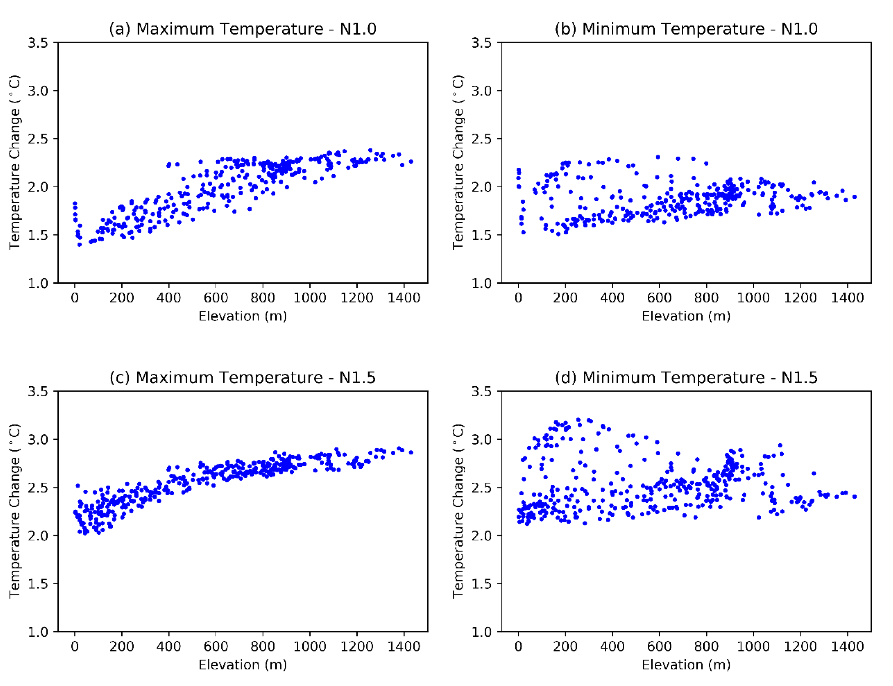
4.2. Projected Changes in Maximum and Minimum Temperatures

Multi-model means of projected changes in annual mean of maximum temperature from the N1.0, N1.5 and N1.X simulations are shown in Figure 4. Changes in maximum temperature show similar spatial distribution between N1.0 and N1.5, with stronger warming on the Australian Alps than surrounding areas (the coastal and inland areas) (Figure 4a,c). About 2–2.5 °C and 2.5–3 °C increase is projected in N1.0 and N1.5 respectively. Larger increase in maximum temperature in N1.5 than N1.0 is due to hotter GCMs used in N1.5 (Figure S5). N1.5 was designed to complement N1.0, hotter CMIP 5 GCMs were selected to use in N1.5 in combination with selected CMIP3 GCMs in N1.0 to cover the overall space of possible future changes in temperature and precipitation [35]. The combination of N1.0 and N1.5, which is N1.X, represents possible future change, which also show larger increases in maximum temperature along the Australian Alps than surrounding areas, with largest increases over the high elevation area (Figure 4e).
Significant increase in minimum temperature is also projected for the Australian Alps and surrounding areas (Figure 4b,d,f), however, largest increase is projected along the eastern coast even if Australian Alps also have larger increase than inland areas. These results indicate that future change in maximum temperature is faster than change in minimum temperature, especially for the Australian Alps.
Future changes in maximum and minimum temperatures with respect to elevation for N1.0 and N1.5 are shown in Figure 5. It is evident that change in maximum temperature is elevation dependent, with larger increase for higher elevation areas (Figure 5a,c). In contrast, change in minimum temperature does not show clear increasing trend with elevation (Figure 5b,d). The changes in maximum and minimum temperatures for N1.5 are larger than those for N1.0.
Furthermore we compared the N1.5 150-year timeseries of anomalies (reference period- 1990–2009) of maximum and minimum temperatures with N1.0 (Figure 6). The N1.5 maximum temperature timeseries aligns well with the N1.0 epochs and adequately fills the temporal gaps, however N1.5 simulations project larger warming compared to N1.0 simulations for high and low elevation for the near future (2020–2039) and the far future (2060–2079). Differences in temperature between N1.0 and N1.5 for 2020–2039 is about 0.2 °C, but it become more than 0.5 °C for 2060–2079. Negligible differences in maximum temperature are seen between high and low elevation before 2010s. The difference starts to increase after 2020s and accelerates after 2060s (Figure 6a). Minimum temperature anomaly is almost identical for high and low elevation for N1.0 and N1.5. However, N1.5 projects stronger minimum temperature increases than N1.0 (Figure 6b).
Projected seasonal changes in maximum temperatures for 2060–2079 relative to 1990–2009 are shown in Figure 7. Larger increases in maximum temperature are projected for southeast Australian in summer and spring than Autumn and Winter, however, faster warming for Australian Alps compared to surrounding areas is seen in Winter when the largest increase is over the top of the Alps (Figure 7c,g). Compared to N1.0, N1.5 projected more intense warming over the Alps in Winter.
Like maximum temperature, minimum temperature is also projected to increase more in Summer and Spring for southeast Australia (Figure S6), but the Alps does not show clearly faster warming for minimum temperature than surrounding areas in any seasons.
As shown in Figure S5, combination of N1.0 and N1.5 selected GCMs generally covered the future change space of the entire CMIP5 ensemble (RCP8.5), then the combined N1.X ensemble can offer an improved sampling of uncertainty in future change. However, we should acknowledge that CMIP3 GCMs are quite different from CMIP5 GCMs in terms of modelling and emission scenario. As discussed before, past studies have shown that for key climate variables, both CMIP3 and CMIP5 GCMs roughly project similar future changes in the highest emission scenario [47,48]. Based on these results CMIP3 and CMIP5 GCMs for the highest emission scenario can be combined into expanded ensemble.

4.3. Projected Changes in Temperature Extremes

Like mean maximum and minimum temperatures, the majority of temperature extremes are also projected to significantly change in future. For example, TNlt2, TN90P, TX90P, TNn and WSDI show clearly larger changes for the Australian Alps than the surrounding areas (Figure 8).
Both N1.0 and N1.5 project future decreases in cold spell duration (CSDI). However, those decreases are not statistically significant (Figure 8a,g). Similarly, Both N1.0 and N1.5 also project decreases in Tnlt2 for southeast Australia. These decreases are significant and elevation dependent (Figure 8b,h). N1.0 and N1.5 project more than 50 and 70 days decreases in TNlt2, respectively. Larger decrease in TNlt2 can be observed over the higher elevation Alps than surrounding areas.
Both N1.0 and N1.5 project significant increase in numbers of warm nights (TN90p) and warm days (TX90p). N1.0 projects more than 9 warm nights increase for southeast Australia and more than 15 warm nights increase for Australian Alps (Figure 8c). N1.5 generally projects more warm nights than N1.0, with more than 12 warm nights increase for southeast Australia and more than 18 warm nights increase for Australian Alps (Figure 8i). Similarly, N1.0 and N1.5 project more than 10 and 15 warm days increase for southeast Australia and more than 20 and 25 warm days increase for the Australian Alps (Figure 8d,j), respectively. The increase in warm days is clearly elevation dependent, while the increase in warm night is elevation dependent but not as strongly as the increase in warm days.
For TNn, N1.0 projects 1.6–2.0 °C increase over southeast Australia, and 2.0–2.4 °C increase over Australian Alps. More than 2.4 °C increase is projected for top of the Alps (Figure 8e). N1.5 projects larger increase in TNn than N1.0, with 2.0–2.4 °C increase in TNn for southeast Australia, and 2.4–2.8 °C increase in TNn for the Alps, even larger increase (more than 2.8 °C) for top of the Alps (Figure 8k). These results suggest largest increase in TNn for the Alps than surrounding areas and the increase is elevation dependent. For WSDI, 0–20 days increases are projected for southeast Australia in N1.0, 20–30 days increases for the Alps and more than 30 days increase for top of the Alps (Figure 8f). N1.5 projects larger increase in WSDI than N1.0, with 20–30 days increase for southeast Australia, 30–40 days increases for the Alps and more than 40 days increases for top of the Alps (Figure 8l). Like TNn, the changes in WSDI are also found to be elevation dependent.

5. Discussion

In this study, we use observed maximum and minimum temperature from AGCD and simulated maximum and minimum temperature from N1.0 and N1.5 to assess changes in temperature over Australian Alps region.
Observed maximum and minimum temperature are taken from AGCD [38], which is obtained by interpolating the data at stations onto a grid. There are not many stations over the Australian Alps, especially for the high elevation areas, which would result in substantial uncertainties in the gridded temperature and precipitation. However, temperature is not as localised as precipitation, and we use mean temperature over grids above and below 1200 m to represent temperature for high and low elevation, which minimise the impact of uncertainties due to sparse temperature monitoring stations over high elevation.
Both N1.0 and N1.5 simulations project significant future warming over Australian Alps, however, the magnitude of changes in maximum and minimum temperature, and temperature extremes for the N1.5 simulations is larger than that of the N1.0 simulations, even if the spatial patterns of future changes are comparable. These major differences can be partly explained by the driving GCMs in N1.0 and N1.5 simulations and the higher emission scenario used in these simulations. The CMIP5 GCMs in N1.5 are hotter than those CMIP3 GCMs in N1.0 [35] (Figure S5).
This paper also presented combined results of N1.0 and N1.5 (N.1X) for the future mean maximum and minimum temperature and its extremes. N1.X projections demonstrate the complementary utility of N1.5 with the original N1.0 and the underlying objective that N1.5 simulations do not replace N1.0 simulations, rather, these updated and enhanced simulations complement N1.0 simulations by expanding the future change space covered by the simulations. Compared to CMIP3 GCMs in N1.0, all CMIP5 GCMs in N1.5 projected a hotter future expanding the future change space of the CMIP3 GCMs (Figure S7). Together N1.0 and N1.5 provide a more complete sampling of this combined future change space. However, it should be noted that N1.0 and N1.5 are driven by GCMs from different generation of CMIP, and emission scenarios used in N1.0 and N1.5 are not the same.
Due to clear cold biases in N1.0 and N1.5 simulations [35], bias-corrected temperature instead of original simulated temperature was used to assess future changes in temperature and its extremes. Bias-corrected temperature is better for calculating threshold related indices such as TNlt2, however, bias-correction also brings some uncertainties as future climate projections are corrected using present climate correction factors. It is not always accurate to assume that present climate biases will be maintained in time.
Elevation dependent warming (EDW) was identified and assessed in multiple studies over the Tibetan Plateau [49,50]. Some mechanisms such as surface albedo feedback, cloud feedback, aerosol radiative forcing and free tropospheric warming, are suggested to explain the phenomenon [51,52,53,54]. Surface albedo feedback (SAF) is considered as a key driver for EDW [53,55,56]. Therefore, we assess future changes in albedo in N1.0 and N1.5 for the Australian Alps which show significant decrease in albedo in cold seasons, especially in winter (Figure 9). The largest decrease in albedo is mostly caused by significant decrease in snow depth and snow cover during the cold season [37]. The changes in maximum temperature have stronger correlation with changes in albedo than changes in minimum temperature, which is as expected as incoming shortwave radiation, which is directly affected by albedo, only occurs during the day when maximum temperatures generally occur. These results align with the finding of previous study of Rangwala et al., 2013 [57]. The Australian Alpine region is much smaller than the Tibetan Plateau, and elevation of Australian Alps is also much lower, however, similar EDW can be seen in N1.0 and N1.5 future projections which indicate mechanism to cause EDW might be similar. Other possible changes in atmosphere circulations and precipitation might also contribute to the changes in temperature over the region. In winter, mid-latitude weather systems are projected to shift south and the westerlies are projected to strengthen. Concurrent and related changes in various measures of mid-latitude circulation are projected, including a more positive Southern Annular Mode, and a decrease in the number of fronts in southern Australia, which result in decrease in projected precipitation over Australian Alps [37] that might contribute to the temperature warming over the region. Further analyses are required to assess contribution from different drivers to result in EWD.
The faster warming and decrease in snow cover extent and snow depths will substantially increase threats for Australian Alps such as loss of biodiversity, increase in pest and weeds, changes in demand for tourism activities and increase costs to maintain ski business. The finding from the study can be used for making relevant policies to minimise the impacts.

6. Conclusions

This paper assessed observed changes in maximum and minimum temperature over the Australian Alps. The observations show that maximum temperature increases at a faster rate for the Alps than minimum temperature, and it also increases at a faster rate for the high elevation areas compared to the surrounding low elevation areas.
This paper also presents future projections of maximum and minimum temperature and temperature extremes for N1.0 and N1.5 under high emissions scenarios. We show that N1.0 and N1.5 project similar patterns of changes in temperature and its extremes even if the magnitude of changes is different. Those differences in temperature and temperature extremes between N1.0 and N1.5 are partially related to differences between the driving GCMs. The combined future projections of both N1.0 and N1.5 (N1.X) provide a more complete sampling of the future change space. However, there are some limitations of combining CMIP3 SRES A2 and CMIP5 RCP8.5 projections due to variations in the driving emissions.
N1.X projects larger increase in maximum temperature over the Australian Alps than the surrounding low elevation areas, especially in winter. Changes in minimum temperature are not as large as changes in maximum temperature. Temperature extremes such as, TNlt2, TN90P, TX90P, TNn and WSDI are projected to significantly increase over the Australian Alps than surrounding areas. This implies that Australian Alps will warm much faster than surrounding areas under future climate.
The results of this study have broad implications for important decision-making processes in the context of climate change adaptation. The outcomes of this work form a baseline for short-, medium- and long-term responses to temperature increases and the facilitation of effective and responsive climate-resilient planning over the Australian Alps.

Supplementary Materials

The following supporting information can be downloaded at: https://www.mdpi.com/article/10.3390/atmos13101686/s1. Figure S1: Domains used in NARCliM1.0 and NARCliM1.5; Figure S2: Anomaly of annual mean maximum and minimum temperatures and their trend for recent three decades (1990s-2010s); Figure S3: Scatter plots of seasonal mean maximum temperature at higher elevation and lower elevation for 1950–2019; Figure S4. Scatter plots of seasonal mean minimum temperature at higher elevation and lower elevation for 1950–2019; Figure S5: Scatter plot of future change (differences between 2060–2079 and 1990–2009) in rainfall and temperature over the land part of the NARCliM domain for 34 CMIP5 and 14 CMIP3 GCMs that passed the performance test; Figure S6: Projected changes in seasonal mean minimum temperature for N1.0, N1.5 and N1.x for 2060–2079 relative to 1990–2009; Figure S7: Projected seasonal changes in TNn for N1.0, N1.5 and N1.x for 2060–2079 relative to 1990–2009; Table S1: The model configuration for the three independent RCMs.

Author Contributions

Conceptualization, F.J., J.P.E. and A.D.L.; methodology, F.J. and N.N.; software, N.N. and E.T.; validation, F.J., J.P.E. and A.D.L.; formal analysis, F.J. and N.N.; investigation, F.J. and K.K.W.C.; resources, E.T.; data curation, E.T.; writing—original draft preparation, F.J. and N.N.; writing—review and editing, All; visualization, N.N.; supervision, G.D.V. and K.B.; project administration, K.B.; funding acquisition, M.L.R. All authors have read and agreed to the published version of the manuscript.

Funding

This research was funded by NSW Climate Change Fund and Australian Research Council Centre of Excellence for Climate Extremes (CE170100023).

Institutional Review Board Statement

Not applicable.

Informed Consent Statement

Not applicable.

Data Availability Statement

NARCliM1.0 and NARCliM1.5 data that support the findings of this study are currently available publicly via the NSW Climate Data Portal (https://climatedata-beta.environment.nsw.gov.au/, accessed on 10 September 2022). Details about AGCD are available at the Australian Bureau of Meteorology website (http://www.bom.gov.au/metadata/catalogue/19115/ANZCW0503900567). The dataset is available on the the NCI (National Computational Infrastructure) server in project zv2. Detail on how to access the data can be found http://climate-cms.wikis.unsw.edu.au/AGCD.

Acknowledgments

This work is made possible by funding from the NSW Climate Change Fund for NSW and Australian Regional Climate Modelling (NARCliM) Project. The modelling work was undertaken on the National Computational Infrastructure (NCI) high performance computers in Canberra, Australia, which is supported by the Australian Commonwealth Government. We thank the climate modelling groups for producing and making available their model outputs, the Earth System Grid Federation (ESGF) for archiving the data and providing access, and the multiple funding agencies who support CMIP3, CMIP5 and the Earth System Grid Federation (ESGF). J.P. Evans acknowledges the support of the Australian Research Council Centre of Excellence for Climate Extremes (CE170100023) and the Climate Systems Hub of the Australian Governments National Environmental Science Program.

Conflicts of Interest

The authors declare no conflict of interest.

References

  1. Hughes, L. Climate change and Australia: Trends, projections and impacts. Austral Ecol. 2003, 28, 423–443. [Google Scholar] [CrossRef]
  2. Brereton, R.; Bennett, S.; Mansergh, I. Enhanced greenhouse climate change and its potential effect on selected fauna of south-eastern Australia: A trend analysis. Biol. Conserv. 1995, 72, 339–354. [Google Scholar] [CrossRef]
  3. Pickering, C.; Armstrong, T. The potential impacts of climate change on plant communities in the Kosciuszko alpine zone. Victorian Nat. 2003, 120, 15–23. [Google Scholar]
  4. NIEIR. The Economic Significance of the Australian Alpine Resorts—Summary Report. 2006; Prepared for: Alpine Resorts Co-ordinating Council. Available online: https://www.arcc.vic.gov.au/uploads/publications-and-research/2011-EconomicSignificanceStudy-FullReport.pdf (accessed on 10 September 2022).
  5. Brown, R.D.; Mote, P.W. The response of Northern Hemisphere Snow covers to a change climate. J. Clim. 2009, 22, 2124–2145. [Google Scholar]
  6. Thompson, J. A MODIS-derived snow climatology (2000–2014) for the Australian Alps. Clim. Res. 2016, 68, 25–38. [Google Scholar] [CrossRef] [Green Version]
  7. Nicholls, N. Climate variability, climate change and the Australian snow season. Aust. Meteorol. Mag. 2005, 54, 177–185. [Google Scholar]
  8. Hennessy, K.J.; Whetton, P.H.; Walsh, K.; Smith, I.N.; Bathols, J.M.; Hutchinson, M.; Sharples, J. Climate change effects on snow conditions in mainland Australia and adaptation at ski resorts through snowmaking. Clim. Res. 2008, 35, 255–270. [Google Scholar] [CrossRef] [Green Version]
  9. Davis, C.J. Towards the development of long-term winter records for the snowy mountains. Aust. Meteorol. Oceanogr. J. 2013, 63, 303–314. [Google Scholar] [CrossRef]
  10. Rasouli, A.A.; Cheung, K.K.W.; Mohammadzadeh Alajujeh, K.; Ji, F. On the Detection of Snow Cover Changes over the Australian Snowy Mountains Using a Dynamic OBIA Approach. Atmosphere 2022, 13, 826. [Google Scholar] [CrossRef]
  11. Bormann, K.J.; McCabe, M.F.; Evans, J.P. Satellite based observations for seasonal snow cover detection and characterisation in Australia. Remote Sens. Environ. 2012, 123, 57–71. [Google Scholar]
  12. Whetton, P.; Haylock, M.; Galloway, R. Climate change and snow-cover duration in the Australian Alps. Clim. Change 1996, 32, 447–479. [Google Scholar] [CrossRef]
  13. Evans, J.P.; Ji, F.; Lee, C.; Smith, P.; Argüeso, D.; Fita, L. Design of a regional climate modelling projection ensemble experiment—NARCliM. Geosci. Model Dev. 2014, 7, 621–629. [Google Scholar] [CrossRef] [Green Version]
  14. Ji, F.; Evans, J.P.; Teng, J.; Scorgie, Y.; Argüeso, D.; Di Luca, A. Evaluation of long-term precipitation and temperature Weather Research and Forecasting simulations for southeast Australia. Clim. Res. 2016, 67, 99–115. [Google Scholar] [CrossRef] [Green Version]
  15. Fita, L.; Evans, J.P.; Argüeso, D.; Liu, Y. Evaluation of the regional climate response in Australia to large-scale climate models in the historical NARCliM simulations. Clim. Dyn. 2016, 49, 2815–2829. [Google Scholar] [CrossRef]
  16. Di Luca, A.; Argüeso, D.; Evans, J.P.; de Elía, R.; Laprise, R. Quantifying the overall added value of dynamical downscaling and the contribution from different spatial scales. J. Geophys. Res. Atmos. 2016, 121, 1575–1590. [Google Scholar] [CrossRef] [Green Version]
  17. Cortés-Hernández, V.E.; Zheng, F.; Evans, J.P. Evaluating regional climate models for simulating sub-daily rainfall extremes. Clim. Dyn. 2015, 47, 1613–1628. [Google Scholar] [CrossRef]
  18. Bao, J.; Sherwood, S.C.; Alexander, L.V.; Evans, J.P. Future increases in extreme precipitation exceed observed scaling rates. Nat. Clim. Change 2017, 7, 128–132. [Google Scholar] [CrossRef]
  19. Ji, F.; Evans, J.P.; Argueso, D.; Fita, L.; Di Luca, A. Using large-scale diagnostic quantities to investigate change in East Coast Lows. Clim. Dyn. 2015, 45, 2443–2453. [Google Scholar] [CrossRef]
  20. Pepler, A.S.; Di Luca, A.; Ji, F.; Alexander, L.V.; Evans, J.P.; Sherwood, S.C. Projected changes in east Australian midlatitude cyclones during the 21st century. Geophys. Res. Lett. 2016, 43, 334–340. [Google Scholar] [CrossRef]
  21. Di Luca, A.; Evans, J.P.; Pepler, A.; Alexander, L.V.; Argueso, D. Australian East Coast Lows in a Regional Climate Model ensemble. J. South. Hemisph. Earth Syst. Sci. 2016, 66, 108–124. [Google Scholar] [CrossRef]
  22. Clarke, H.; Pitman, A.J.; Kala, J.; Carouge, C.; Haverd, V.; Evans, J.P. An investigation of future fuel load and fire weather in Australia. Clim. Change 2016, 139, 591–605. [Google Scholar] [CrossRef] [Green Version]
  23. Clarke, H.; Evans, J.P. Exploring the future change space for fire weather in southeast Australia. Theor. Appl. Climatol. 2019, 136, 513–527. [Google Scholar] [CrossRef] [Green Version]
  24. Di Virgilio, G.; Evans, J.P.; Blake, S.A.P.; Armstrong, M.; Dowdy, A.J.; Sharples, J.; McRae, R. Climate Change Increases the Potential for Extreme Wildfires. Geophys. Res. Lett. 2019, 46, 8517–8526. [Google Scholar] [CrossRef]
  25. Evans, J.P.; Kay, M.; Prasad, A.; Pitman, A. The resilience of Australian wind energy to climate change. Environ. Res. Lett. 2018, 13, 024014. [Google Scholar] [CrossRef]
  26. Ji, F.; Evans, J.P.; Di Luca, A.; Jiang, N.B.; Olson, R.; Fita, L.; Argueso, D.; Chang, L.T.-C.; Scorgie, Y.; Riley, M. Projected change in characteristics of near surface temperature inversions for Southeast Australia. Clim. Dyn. 2018, 52, 1487–1503. [Google Scholar] [CrossRef]
  27. Ji, F.; Evans, J.P.; Di Virgilio, G.; Nishant, N.; Di Luca, A.; Herold, N.; Downes, S.M.; Tam, E.; Beyer, K. Projected changes in vertical temperature profiles for Australasia. Clim. Dyn. 2020, 55, 2453–2468. [Google Scholar] [CrossRef]
  28. Argüeso, D.; Evans, J.P.; Fita, L.; Bormann, K.J. Temperature response to future urbanization and climate change. Clim. Dyn. 2014, 42, 2183–2199. [Google Scholar] [CrossRef]
  29. Argüeso, D.; Evans, J.P.; Pitman, A.J.; Di Luca, A. Effects of city expansion on heat stress under climate change conditions. PLoS ONE 2015, 10, e0117066. [Google Scholar] [CrossRef] [PubMed]
  30. Macadam, I.; Argüeso, D.; Evans, J.P.; Liu, D.L.; Pitman, A.J. The effect of bias correction and climate model resolution on wheat simulations forced with a regional climate model ensemble. Int. J. Climatol. 2016, 36, 4577–4591. [Google Scholar] [CrossRef] [Green Version]
  31. Liu, D.L.; Wang, B.; Evans, J.; Ji, F.; Waters, C.; Macadam, I.; Beyer, K. Propagation of climate model biases to biophysical modelling can complicate assessments of climate change impact in agricultural systems. Int. J. Climatol. 2019, 39, 424–444. [Google Scholar] [CrossRef] [Green Version]
  32. Wang, B.; Liu, D.L.; Evans, J.P.; Ji, F.; Waters, C.; Macadam, I.; Beyer, K. Modelling and evaluating the impacts of climate change on three major crops in south-eastern Australia using regional climate model simulations. Theor. Appl. Climatol. 2019, 138, 509–526. [Google Scholar] [CrossRef]
  33. Evans, J.P.; Argueso, D.; Olson, R.; Di Luca, A. Bias-corrected regional climate projections of extreme rainfall in south-east Australia. Theor. Appl. Climatol. 2017, 130, 1085–1098. [Google Scholar] [CrossRef]
  34. Herold, N.; Downes, S.M.; Gross, M.H.; Ji, F.; Nishant, N.; Macadam, I.; Ridder, N.N.; Beyer, K. Projected changes in the frequency of climate extremes over southeast Australia. Environ. Res. Commun. 2021, 3, 011001. [Google Scholar] [CrossRef]
  35. Nishant, N.; Evans, J.P.; Di Virgilio, G.; Downes, S.M.; Ji, F.; Cheung, K.K.W.; Tam, E.; Miller, J.; Beyer, K.; Riley, M.L. Introducing NARCliM1.5: Evaluating the Performance of Regional Climate Projections for Southeast Australia for 1950–2100. Earth’s Future 2021, 9, e2020EF001833. [Google Scholar] [CrossRef]
  36. Ji, F.; Nishant, N.; Evans, J.P.; Di Virgilio, G.; Cheung, K.K.W.; Tam, E.; Beyer, K.; Riley, M.L. Introducing NARCliM1.5: Evaluation and Projection of Climate Extremes for Southeast Australia. Weather. Clim. Extrem. 2022. Under Review. [Google Scholar] [CrossRef]
  37. Di Luca, A.; Evans, J.P.; Ji, F. Australian snowpack in the NARCliM ensemble: Evaluation, bias correction and future projections. Clim. Dyn. 2018, 51, 639–666. [Google Scholar] [CrossRef]
  38. Evans, A.; Jones, D.; Smalley, R.; Lellyett, S. An enhanced Gridded Rainfall Analysis Scheme for Australia. Bureau Research Report (41); 2020. Available online: http://www.bom.gov.au/research/publications/researchreports/BRR-041.pdf (accessed on 10 September 2022).
  39. Skamarock, W.C.; Klemp, J.B. A time-split nonhydrostatic atmospheric model for weather research and forecasting applications. J. Comput. Phys. 2008, 227, 3465–3485. [Google Scholar] [CrossRef]
  40. Evans, J.P.; Ekström, M.; Ji, F. Evaluating the performance of a WRF physics ensemble over South-East Australia. Clim. Dyn. 2012, 39, 1241–1258. [Google Scholar] [CrossRef]
  41. Ji, F.; Ekström, M.; Evans, J.P.; Teng, J. Evaluating rainfall patterns using physics scheme ensembles from a regional atmospheric model. Theor. Appl. Climatol. 2014, 115, 297–304. [Google Scholar] [CrossRef]
  42. Evans, J.P.; Ji, F.; Abramowitz, G.; Ekström, M. Optimally choosing small ensemble members to produce robust climate simulations. Environ. Res. Lett. 2013, 8, 044050. [Google Scholar] [CrossRef] [Green Version]
  43. Di Virgilio, G.; Evans, J.P.; Di Luca, A.; Olson, R.; Argüeso, D.; Kala, J.; Andrys, J.; Hoffmann, P.; Katzfey, J.J.; Rockel, B. Evaluating reanalysis-driven CORDEX regional climate models over Australia: Model performance and errors. Clim. Dyn. 2019, 53, 2985–3005. [Google Scholar] [CrossRef]
  44. Alexander, L.V.; Herold, N. Climpactv2 Indices and Software. A Document Prepared on behalf of the Commission for Climatology (CCL) Expert Team on Sector-Specific Climate Indices (ET-SCI). 2015. Available online: https://epic.awi.de/id/eprint/49274/1/ClimPACTv2_manual.pdf (accessed on 10 September 2022).
  45. Zivin, J.G.; Shrader, J. Temperature extremes, health, and human capital. Future Child. 2016, 26, 31–50. [Google Scholar] [CrossRef]
  46. Tebaldi, C.; Arblaster, J.M.; Knutti, R. Mapping model agreement on future climate projections. Geophys. Res. Lett. 2011, 38, 23. [Google Scholar] [CrossRef]
  47. Knutti, R.; Sedláček, J. Robustness and uncertainties in the new CMIP5 climate model projections. Nat. Clim. Change 2013, 3, 369–373. [Google Scholar] [CrossRef]
  48. Moise, A.F.; Wilson, L.; Grose, M.; Whetton, P.; Watterson, I.; Bhend, J.; Bathols, J.; Hanson, L.; Erwin, T.; Bedin, T.; et al. Evaluation of CMIP3 and CMIP5 Models over the Australian Region to Inform Confidence in Projections. Aust. Meteorol. Oceanogr. J. 2015, 65, 19–53. [Google Scholar] [CrossRef]
  49. Gao, Y.; Leung, L.R.; Zhang, Y.; Cuo, L. Changes in moisture flux over the Tibetan Plateau during 1979–2011: Insights from a high-resolution simulation. J. Clim. 2015, 28, 4185–4197. [Google Scholar] [CrossRef]
  50. Nengker, T.; Choudhary, A.; Dimri, A.P. Assessment of the performance of CORDEX-SA experiments in simulating seasonal mean temperature over the Himalayan region for the present climate: Part I. Clim. Dyn. 2018, 50, 2411–2441. [Google Scholar] [CrossRef]
  51. Rangwala, I.; Miller, J.R.; Russell, G.L.; Xu, M. Using a global climate model to evaluate the influences of water vapor, snow cover and atmospheric aerosol on warming in the Tibetan Plateau during the twenty-first century. Clim. Dyn. 2010, 34, 859–872. [Google Scholar] [CrossRef]
  52. Rangwala, I.; Miller, J.R. Climate change in mountains: A review of elevation-dependent warming and its possible causes. Clim. Change 2012, 114, 527–547. [Google Scholar] [CrossRef]
  53. Yan, L.; Liu, Z.; Chen, G.; Kutzbach, J.E.; Liu, X. Mechanisms of elevation-dependent warming over the Tibetan plateau in quadrupled CO2 experiments. Clim. Change 2016, 135, 509–519. [Google Scholar] [CrossRef]
  54. You, Q.; Chen, D.; Wu, F.; Pepin, N.; Ahrens, B.; Jiang, Z.; Wu, Z.; Kang, S.; AghaKouchak, A. Elevation dependent warming over the Tibetan Plateau: Patterns, mechanisms and perspectives. Earth-Sci. Rev. 2020, 210, 103349. [Google Scholar] [CrossRef]
  55. Giorgi, F.; Hurrell, J.W.; Marinucci, M.R.; Beniston, M. Elevation dependency of the surface climate change signal: A model study. J. Clim. 1997, 10, 288–296. [Google Scholar] [CrossRef]
  56. Minder, J.R.; Letcher, T.W.; Liu, C.H. The character and causes of elevation-dependent warming in high-resolution simulations of Rocky Mountain climate change. J. Clim. 2018, 31, 2093–2113. [Google Scholar] [CrossRef]
  57. Rangwala, I.; Sinsky, E.; Miller, J.R. Amplified warming projections for high altitude regions of the northern hemisphere mid-latitudes from CMIP5 models. Environ. Res. Lett. 2013, 8, 024040. [Google Scholar] [CrossRef] [Green Version]
Figure 1. Locations of Australian Alps. The blue rectangle area is the domain to analyse differences between high and low elevations. The red rectangle area denotes the domain to show spatial distribution of future changes in temperature and its extremes.
Atmosphere 13 01686 g001
Figure 2. Anomaly of observed (AGCD) annual mean of maximum and minimum temperature and their trends for Australian Alps. The trends are statistically significant using a non-parametric Mann-Kendall test at the 95% confidence level.
Atmosphere 13 01686 g002
Figure 3. Plots of annual mean maximum (a) and minimum (b) temperatures for high and low elevation for 1950–2019. The trends are statistically significant using a non-parametric Mann-Kendall test at the 95% confidence level.
Atmosphere 13 01686 g003
Figure 4. Projected changes in annual mean of maximum and minimum temperatures for N1.0, N1.5 and N1.x for 2060–2079 relative to 1990–2009 (unit: °C). Stippling indicates statistically significant changes using a non-parametric Mann-Kendall test at the 95% confidence level. The black solid lines are the 1200 m contour where the high elevation areas are.
Atmosphere 13 01686 g004
Figure 5. Scatter plot of future changes in maximum and minimum temperatures for 2060–2079 relative to 1990–2009 vs. elevation. Here each dot represents multi-model mean future change in maximum and minimum temperature for N1.0/N1.5 respectively for a NARCliM grid cell over the Alpine region.
Atmosphere 13 01686 g005
Figure 6. Time series (from 1951–2099) of maximum and minimum temperatures anomalies (calculated with respect to 1990–2009) for high and low elevation for N1.0 and N1.5. Here red and blue solid lines denote the ensemble mean of NARCliM1.5 (N1.5) simulations for high and low elevation respectively, brown, and green solid lines represent the ensemble mean of NARCliM (N1.0) simulations for high and low elevation respectively. The shading denotes the max and min across the ensemble members.
Atmosphere 13 01686 g006
Figure 7. Projected seasonal changes in maximum temperature for N1.0, N1.5 and N1.x for 2060–2079 relative to 1990–2009. Stippling indicates statistically significant changes using a non-parametric Mann-Kendall test at the 95% confidence level. The black solid lines are the 1200 m contour where the high elevation areas are.
Atmosphere 13 01686 g007
Figure 8. Projected changes in annual CSDI, TNlt2, TN90P, TX90P, TNn and WSDI for N1.0, N1.5 and N1.x for 2060–2079 relative to 1990–2009. Stippling indicates statistically significant changes using a non-parametric Mann-Kendall test at the 95% confidence level. The black solid lines are the 1200 m contour where the high elevation areas are.
Atmosphere 13 01686 g008
Figure 9. Future changes in mean seasonal albedo for 2060–2079 relative to 1990–2009 for N1.0, N1.5 and N1.x. Stippling indicates statistically significant changes using a non-parametric Mann-Kendall test at the 95% confidence level. The black solid lines are the 1200 m contour where the high elevation areas are.
Atmosphere 13 01686 g009
Table 1. NARCliM1.0 and NARCliM1.5 simulations used in this study. Here for clarity, blue and orange colours differentiate between N1.0 and N1.5 simulations.
Simulation-NameDriving GCMRCMWRF VersionHistorical PeriodFuture PeriodsCMIP Future Pathway
CGCM3.1-R1CGCM3.1R1WRF3.31990–20092020–2039; 2060–2079SRES A2
CGCM3.1-R2CGCM3.1R2WRF3.31990–20092020–2039; 2060–2079SRES A2
CGCM3.1-R3CGCM3.1R3WRF3.31990–20092020–2039; 2060–2079SRES A2
MK3.0-R1Mk3.0R1WRF3.31990–20092020–2039; 2060–2079SRES A2
MK3.0-R2Mk3.0R2WRF3.31990–20092020–2039; 2060–2079SRES A2
MK3.0-R3Mk3.0R3WRF3.31990–20092020–2039; 2060–2079SRES A2
ECHAM5-R1ECHAM5R1WRF3.31990–20092020–2039; 2060–2079SRES A2
ECHAM5-R2ECHAM5R2WRF3.31990–20092020–2039; 2060–2079SRES A2
ECHAM5-R3ECHAM5R3WRF3.31990–20092020–2039; 2060–2079SRES A2
MIROC-R1MIROCR1WRF3.31990–20092020–2039; 2060–2079SRES A2
MIROC-R2MIROCR2WRF3.31990–20092020–2039; 2060–2079SRES A2
MIROC-R3MIROCR3WRF3.31990–20092020–2039; 2060–2079SRES A2
CanESM2-R1CanESM2R1WRF3.61951–20052006–2100RCP8.5
CanESM2-R2CanESM2R2WRF3.61951–20052006–2100RCP8.5
ACCESS1-0-R1ACCESS1-0R1WRF3.61951–20052006–2100RCP8.5
ACCESS1-0-R2ACCESS1-0R2WRF3.61951–20052006–2100RCP8.5
ACCESS1-3-R1ACCESS1-3R1WRF3.61951–20052006–2100RCP8.5
ACCESS1-3-R2ACCESS1-3R2WRF3.61951–20052006–2100RCP8.5
Table 2. List of ET-SCI Indices assessed in this study.
NoIndexDefinitionUnitsTimescaleSectors
1.CSDICold spell duration indicator (Annual count of days with at least 6 or more consecutive days when minimum temperature < 10th percentile)daysAnnualHealth, agriculture and food security, coasts, disaster risk reduction, energy, fisheries, forestry/GHGs, cryosphere
2.TNlt2Number of days when minimum temperature below 2 °CdaysMonthly/AnnualAgriculture and food security, forestry/GHGs, cryosphere
3.TN90pNumber of warm nightsdaysAnnualEnergy
4.TX90pNumber of warm daysdaysAnnualEnergy
5.WSDIWarm spell duration indicator (Annual number of days contributing to events where 6 or more consecutive days experience maximum temperature > 90th percentile)daysAnnualHealth, agriculture and food security, water resources and food security, coasts, disaster risk reduction, energy, fisheries, forestry/GHGs, cryosphere
6.TNnColdest daily minimum temperature°CAnnual/MonthlyAgriculture and food security, energy, forestry/GHGs, cryosphere
Publisher’s Note: MDPI stays neutral with regard to jurisdictional claims in published maps and institutional affiliations.

